


 下吧笑掉
下吧笑掉
范文一:复高斯分布
Equation Chapter 1 Section 1复高斯分布
1.一复复高斯机复量随
如果复机复量随X和Y都服高斯分布~而且是不相复的;复复也是立的,~均复分复复从独和~方差都复mmxy2~复其复合率密度函;概数probability density function~pdf,复,σ
\* MERGEFORMAT ()
复复的复机复量随Z=X+iY复复复高斯机复量。称随Z的均复m和方差 分复复,z
\* MERGEFORMAT ()
\* MERGEFORMAT ()
特殊的~均复当m和m均复0复~xy
随机复量Z复;零均复,循复复复高斯称称(Zero Mean Circular Symmetric Complex Gaussian, ZMCSCG)机复随21量。σ称复Z的每复复复上的方差个数(variance per real dimension)。
复1 二复高斯分布
当虚随复部部机复量都是不相复的高斯RV~且具有相同方差~复复高斯机复量随Z=X+iY的率密度函复,概数
\* MERGEFORMAT ()可以看出~用复部,当i部的方式表示复后~虚来数式和式其复是等同的。但是更加复;更像一“一复”的凑个随概数虚来机复量的率密度函,。但是在复算期望复行复分的复候~复是要复复部部复行复分;利用式,。复也适用于多复复机复量的情。随况
2.复高斯机矢量随
首先复充一下循复复称(Circular Symmetric~或CS)的含复([2], sec 2.6-1),如果复机矢量随Z复足,以任意角度旋复后~所复得的新矢量原矢量有相同的率密度函~复复复机矢量跟概数称随Z复循复复的。 称即,和Z的率概密度函相同。复然~由此定复可以推出,数tE[Z]=0, E[ZZ]=0 \*MERGEFORMAT ()2当Z复高斯机矢量复~循复复件随称条跟等价。特复的~且当Z复一复复~E[Z]=0。
故~复于d复的
高斯机矢量随Z=X+iY (粗表示列矢量体)~其复足当
\* MERGEFORMAT ()t复([2]复复的称Z是proper的,复足即E[(Z-m)( Z-m))] =0)~新机矢量随Z - m 是循复复;复于复机矢称随ZZZ
量~零均复,proper件复复循复复,的~复量代复后的率密度函复条即称概数
\* MERGEFORMAT ()H其中, m=E[z] 是机矢量随z的均复, Σ=E[(z-m)(z-m)] 是互复方差矩复;假复非奇,异, |Σ| 是Σ的行zzz
H列式~ z 表示z的共复复置.
如果复复高斯机矢量个随Z不是proper的~复其率密度函不能复复表示~而复以复复的概数2d复复机矢量的复合分随布表示,来
\* MERGEFORMAT ()
其中
\* MERGEFORMAT ()且。
幸的是~在大多复用复境下~我复都可以假复复机矢量运数随Z
1 实实实实实实实实实实实实实实实实实实实实其里没有必要零均,因由后面循称的定,Z强一定是零均的。实实实
m复循复复的~甚至可以假复称Z本身就是循复复的。称z
当随另两复复高斯机复量取模复~可以得到复特殊的分布,瑞利分布(Rayleigh distribution)和斯分布莱;Rice
,。distribution
复有22高斯机复量随z=x+iy~令a=|E[z]|~σ=E[|z|]~复r=|z|的pdf可以通复坐复复复,x=r cosθ, y=r sinθ, 求复并复分布复得。来
?当a=0复~r的pdf复瑞利分布,
\* MERGEFORMAT ()
?当a>0实,r的pdf实莱斯分布:
\* MERGEFORMAT ()
其中I(.)表示零一修正塞函数,定实实实实实实实实实实实实实实0
\* MERGEFORMAT ()
22莱斯分布常用K因子;斯因子,描述~莱来K=a/2σ。在多无复通信复境中~描述了直射;主,径它径径
的功率散射功率之比。跟径K,0复~r复瑞利分布。K非常大复~r接近高斯分布。在无复信道中~斯分布莱是一复最常复的用于描述接收信包复复复复复特性的分布复型。斯因子是反映信道复量的重要~在复算信道复号莱参数
量和复路复算、移复台移复速度以及复向性能分析等都复复着重要的作用。信在复复复程中由于多效复~接收信号径号
是直复信;主信,和多信的加~此复接收信的包复服斯分布。号径号径号叠号从莱
复2 莱概数斯分布的率密度函
高斯分布在工程上有泛的复用。例如~在通信理复中~高斯白复入接收机后~复复低通复波复理复成窄复高很广噪声
斯~加在解复的信之上~形成一复高斯机复量;正交复制,。噪声叠号个随
注,本文在[1]的基复之上复行复、考了翻并参[2]和[3]复[1]中的描述复行了修改、复充~最复完成。复片均自复。来网
REFERENCES
[1] complex Gaussian distribution, http://everything2.com/title/complex+Gaussian+distributionth[2] J. Proakis, M. Salehi, Digital Communications, 5, McGraw-Hill Company, New York:2008
[3] 莱斯分布,百度百科.
http://baike.baidu.com/link?url=tGSIqleByObem0cjEDAlMzb7Ac_St3L4dS9-b8OgRbzISsiG6WY6LnaUyzr5iCiK
范文二:复高斯分布
复高斯分布
1. 一维复高斯随机变量
如果实随机变量X和Y都服从高斯分布,而且是不相关的(这时也是独立的),均值分别为mx和my,方差都为σ2,则其联合概率密度函数(probability density function,pdf)为:
骣(x-m)2+(y-m)2?xy1??pXY(x,y)=exp-?2s22ps2??è()÷÷÷ (1) ÷÷÷÷?
2对应的复随机变量Z=X+iY则称为复高斯随机变量。Z的均值mz和方差sz 分别为:
mz=E[Z]=E[X+iY]=E[X]+iE[Y]=mx+imy (2)
2*2sz=E轾Z-m?Z-mEX-m+iY-m()()()()zzxy犏臌2 (3) =E轾Y-my)(X-mx)2+E轾(犏犏臌臌
=2s2
特殊的,当均值mx和my均为0时,复随机变量Z称为(零均值)循环对称复高斯(Zero Mean Circular Symmetric Complex Gaussian, ZMCSCG)随机变量1。σ2称为Z的每个实数维上的方差(variance per real dimension)。
图1 二维高斯分布
当实部虚部随机变量都是不相关的高斯RV,且具有相同方差,则复高斯随机变量Z=X+iY的概率密度函数为:
骣z-mz1??pz(z)=exp-?2?2ps桫2s2
骣z-mz1??=exp-?22?szpszè2÷÷÷÷2 (4) ÷÷÷÷?
1 其实这里没有必要强调零均值,因为由后面循环对称的定义,Z一定是零均值的。
可以看出,当用实部+i虚部的方式来表示复数后,(4)式和(1)式其实是等同的。但是更加紧凑(更像一个“一维”的随机变量的概率密度函数)。但是在计算期望进行积分的时候,还是要对实部虚部来进行积分(利用
(1)式)。这也适用于多维复随机变量的情况。
2. 复高斯随机矢量
首先补充一下循环对称(Circular Symmetric,或CS)的含义([2], sec 2.6-1):如果复随机矢量Z满足:以任意角度旋转后,所获得的新矢量跟原矢量有相同的概率密度函数,则称复随机矢量Z为循环对称的。即
E[Z]=0, E[ZZt]=0 (5)
当Z为高斯随机矢量时,循环对称条件跟(5)等价。特别的,且当Z为一维时,E[Z2]=0。
故,对于d维的复高斯随机矢量Z=X+iY (粗体表示列矢量),当其满足
CX=CY,CXY=-CYX (6)
时([2]称这样的Z是proper的,即满足E[(Z-mZ)( Z-mZ)t)] =0),新随机矢量Z - mZ 是循环对称(对于复随机矢量,零均值+proper条件即对应循环对称)的,变量代换后的概率密度函数为
骣(z-mz)HΣ-1(z-mz)÷?÷?p(z)=exp-÷?d÷ 2?(p)Σ桫1(7)
其中, mz=E[z] 是随机矢量z的均值, Σ=E[(z-mz)(z-mz)H] 是互协方差矩阵(假设非奇异), |Σ| 是Σ的行列式, zH 表示z的共轭转置.
如果这个复高斯随机矢量Z不是proper的,则其概率密度函数不能这样表示,而应以对应的2d维实随机矢量的联合分布来表示:
其中
%=[X1,X2,...X Z,dY1,Y2,
z]。 且m%z=E[%tY. . . , d,]p(z)=p(%z)=1t%exp-z-mC%z-m%()%zz(%z) 2(2p)dC%z1{}(8) (9)
幸运的是,在大多数应用环境下,我们都可以假设复随机矢量Z-mz为循环对称的,甚至可以假设Z本身就是循环对称的。
当对复高斯随机变量取模时,可以得到另两种特殊的分布:瑞利分布(Rayleigh distribution)和莱斯分布(Rice distribution)。
设有复高斯随机变量z=x+iy,令a=|E[z]|,σ2=E[|z|2],则r=|z|的pdf可以通过坐标变换:x=r cosθ, y=r sinθ, 并求边缘分布来获得。
·当a=0时,r的pdf为瑞利分布:
骣r÷骣r2÷?÷, r 0 p(r)=?÷exp?-?÷桫2s2÷s2÷?(10)
·当a>0时,r的pdf为莱斯分布:
骣r鼢骣r2+a2÷骣ar?÷p(r)=exp-I, r 0 ?鼢0÷桫2s2÷s2鼢?s2(11)
其中I0(.)表示零阶一类修正贝塞尔函数,定义为
I0(x)=12pexp(xcosq)dq 2pò0(12)
莱斯分布常用K因子(莱斯因子)来描述,K=a2/2σ2。在多径无线通信环境中,它描述了直射径(主径)的功率跟散射径功率之比。K=0时,r为瑞利分布。K非常大时,r接近高斯分布。在无线信道中,莱斯分布是一种最常见的用于描述接收信号包络统计时变特性的分布类型。莱斯因子是反映信道质量的重要参数,在计算信道质量和链路预算、移动台移动速度以及测向性能分析等都发挥着重要的作用。信号在传输过程中由于多径效应,接收信号是直视信号(主径信号)和多径信号的叠加,此时接收信号的包络服从莱斯分布。
图2 莱斯分布的概率密度函数
复高斯分布在工程上有很广泛的应用。例如,在通信理论中,高斯白噪声进入接收机后,经过低通滤波处理变成窄带高斯噪声,叠加在解调的信号之上,形成一个复高斯随机变量(正交调制)。
注:本文在[1]的基础之上进行翻译、并参考了[2]和[3]对[1]中的描述进行了修改、补充,最终完成。图片均来自网络。
REFERENCES
[1] complex Gaussian distribution,
[2] J. Proakis, M. Salehi, Digital Communications, 5th, McGraw-Hill Company, New York:2008
[3] 莱斯分布,百度百科.
http://baike.baidu.com/link?url=tGSIqleByObem0cjEDAlMzb7Ac_St3L4dS9-b8OgRbzISsiG6WY6LnaUyzr5iCiK
范文三:边缘高斯分布
882. PROBABILITY DISTRIBUTIONS 2.3.2Marginal Gaussian distributions
We have seen that if a joint distribution p (x a , x b ) is Gaussian, then the condi-
tional distribution p (x a |x b ) will again be Gaussian. Now we turn to a discussion of
the marginal distribution given by
(2.83)p (x a ) =p (x a , x b ) d x b
which, as we shall see, is also Gaussian. Once again, our strategy for evaluating this
distribution ef?cientlywill be to focus on the quadratic form in the exponent of the
joint distribution and thereby to identify the mean and covariance of the marginal
distribution p (x a ) .
The quadratic form for the joint distribution can be expressed, using the par-
titioned precision matrix, in the form (2.70).Because our goal is to integrate out x b , this is most easily achieved by ?rstconsidering the terms involving x b and then
completing the square in order to facilitate integration. Picking out just those terms
that involve x b , we have
11T ?11?1?1T T Λx +x m =??Λm ) Λ(x ?Λm )+(x m Λbb m (2.84)?x T bb b b bb b b bb bb 2b 22
where we have de?ned
m =Λbb μb ?Λba (x a ?μa ) . (2.85)
We see that the dependence on x b has been cast into the standard quadratic form of a
Gaussian distribution corresponding to the ?rstterm on the right-hand side of (2.84),
plus a term that does not depend on x b (butthat does depend on x a ). Thus, when
we take the exponential of this quadratic form, we see that the integration over x b required by (2.83)will take the form
11?1T exp ?(x b ?Λ?d x b . (2.86)bb m ) Λbb (x b ?Λbb m ) 2
This integration is easily performed by noting that it is the integral over an unnor-
malized Gaussian, and so the result will be the reciprocal of the normalization co-
ef?cient.We know from the form of the normalized Gaussian given by (2.43),that
this coef?cientis independent of the mean and depends only on the determinant of
the covariance matrix. Thus, by completing the square with respect to x b , we can
integrate out x b and the only term remaining from the contributions on the left-hand
side of (2.84)that depends on x a is the last term on the right-hand side of (2.84)in
which m is given by (2.85).Combining this term with the remaining terms
from
2.3. The Gaussian Distribution
(2.70)that depend on x a , we obtain 89
1T 1[Λbb μb ?Λba (x a ?μa )]Λ?bb [Λbb μb ?Λba (x a ?μa )]21T ?x T a Λaa x a +x a (Λaa μa +Λab μb ) +const 21?1=?x T a (Λaa ?Λab Λbb Λba ) x a 2?1?1+x T μa +const (2.87)a (Λaa ?Λab Λbb Λba )
where ‘const’denotes quantities independent of x a . Again, by comparison with
(2.71),we see that the covariance of the marginal distribution of p (x a ) is given by
1?1. Σa =(Λaa ?Λab Λ?bb Λba ) (2.88)
Similarly, the mean is given by
1Σa (Λaa ?Λab Λ?bb Λba ) μa =μa (2.89)
where we have used (2.88).The covariance in (2.88)is expressed in terms of the
partitioned precision matrix given by (2.69).We can rewrite this in terms of the
corresponding partitioning of the covariance matrix given by (2.67),as we did for
the conditional distribution. These partitioned matrices are related by
?1 Λaa Λab Σaa Σab =(2.90)Λba Λbb Σba Σbb
Making use of (2.76),we then have
?1?1Λaa ?Λab Λbb Λba =Σaa . (2.91)
Thus we obtain the intuitively satisfying result that the marginal distribution p (x a )
has mean and covariance given by
E [x a ]=μa
cov[x a ]=Σaa . (2.92)(2.93)
We see that for a marginal distribution, the mean and covariance are most simply ex-
pressed in terms of the partitioned covariance matrix, in contrast to the conditional
distribution for which the partitioned precision matrix gives rise to simpler expres-
sions.
Our results for the marginal and conditional distributions of a partitioned Gaus-
sian are summarized below.
Partitioned Gaussians
Given a joint Gaussian distribution N (x |μ, Σ) with Λ≡Σ?1and x a μa x =, μ=x b μb (2.94)
90
2. PROBABILITY DISTRIBUTIONS
Figure 2.9The plot on the left shows the contours of a Gaussian distribution p (x a , x b ) over two variables, and the plot on the right shows the marginal distribution p (x a ) (bluecurve) and the conditional distribution p (x a |x b ) for x b =0. 7(redcurve).
Σ= Σaa Σab , Σba Σbb Λaa Λab Λ=. Λba Λbb (2.95)
Conditional distribution:
1p (x a |x b ) =N (x |μa |b , Λ?aa ) (2.96)
(2.97)μa |b
Marginal distribution:1=μa ?Λ?aa Λab (x b ?μb ) .
p (x a ) =N (x a |μa , Σaa ) . (2.98)
We illustrate the idea of conditional and marginal distributions associated with
a multivariate Gaussian using an example involving two variables in Figure 2.9.
2.3.3Bayes’theorem for Gaussian variables
In Sections 2.3.1and 2.3.2, we considered a Gaussian p (x ) in which we parti-
tioned the vector x into two subvectors x =(x a , x b ) and then found expressions for
the conditional distribution p (x a |x b ) and the marginal distribution p (x a ) . We noted
that the mean of the conditional distribution p (x a |x b ) was a linear function of x b .
Here we shall suppose that we are given a Gaussian marginal distribution p (x ) and a
Gaussian conditional distribution p (y |x ) in which p (y |x ) has a mean that is a linear
function of x , and a covariance which is independent of x . This is an example of
Exercise 2.292.3. The Gaussian Distribution 91a linear Gaussian model (Roweisand Ghahramani, 1999), which we shall study in greater generality in Section 8.1.4. We wish to ?ndthe marginal distribution p (y ) and the conditional distribution p (x |y ) . This is a problem that will arise frequently in subsequent chapters, and it will prove convenient to derive the general results here. We shall take the marginal and conditional distributions to be p (x ) =N x |μ, Λ?1 p (y |x ) =N y |Ax +b , L ?1 (2.99)(2.100)where μ, A , and b are parameters governing the means, and Λand L are precision matrices. If x has dimensionality M and y has dimensionality D , then the matrix A has size D ×M . First we ?ndan expression for the joint distribution over x and y . To do this, we de?ne z =x y (2.101)and then consider the log of the joint distribution ln p (z ) =ln p (x ) +ln p (y |x ) =?12(x ?μ) T Λ(x ?μ) ?12(y ?Ax ?b ) T L (y ?Ax ?b ) +const (2.102)where ‘const’denotes terms independent of x and y . As before, we see that this is a quadratic function of the components of z , and hence p (z ) is Gaussian distribution. To ?ndthe precision of this Gaussian, we consider the second order terms in (2.102),which can be written as ?1x T (Λ+A T LA ) x ?1y T Ly +1y T LAx +1x T A T 2Ly =?1 x 222T Λ+A T LA ?A T L x 12y ?LA L y =?z T 2Rz (2.103)and so the Gaussian distribution over z has precision (inversecovariance) matrix given by R =Λ+A T LA ?A T L ?LA L . (2.104)The covariance matrix is found by taking the inverse of the precision, which can be done using the matrix inversion formula (2.76)to give
cov[z ]=R ?1=Λ?1Λ?1A T
AΛ?1L ?1+AΛ?1A T . (2.105)
922. PROBABILITY DISTRIBUTIONS
Exercise 2.30
Section 2.3
Section 2.3Similarly, we can ?ndthe mean of the Gaussian distribution over z by identify-ing the linear terms in (2.102),which are given by x T Λμ?x T A T Lb +y T Lb =x T Λμ?A T Lb y Lb . (2.106)Using our earlier result (2.71)obtained by completing the square over the quadratic form of a multivariate Gaussian, we ?ndthat the mean of z is given by E [z ]=R ?1Λμ?A T Lb Lb . (2.107)Making use of (2.105),we then obtain E [z ]=A μμ +b . (2.108)Next we ?ndan expression for the marginal distribution p (y ) in which we have marginalized over x . Recall that the marginal distribution over a subset of the com-ponents of a Gaussian random vector takes a particularly simple form when ex-pressed in terms of the partitioned covariance matrix. Speci?cally,its mean and covariance are given by (2.92)and (2.93),respectively. Making use of (2.105)and (2.108)we see that the mean and covariance of the marginal distribution p (y ) are given by E [y ]=A μ+b (2.109)cov[y ]=L ?1+AΛ?1A T . (2.110)A special case of this result is when A =I , in which case it reduces to the convolu-tion of two Gaussians, for which we see that the mean of the convolution is the sum of the mean of the two Gaussians, and the covariance of the convolution is the sum of their covariances. Finally, we seek an expression for the conditional p (x |y ) . Recall that the results for the conditional distribution are most easily expressed in terms of the partitioned precision matrix, using (2.73)and (2.75).Applying these results to (2.105)and
(2.108)we see that the conditional distribution p (x |y ) has mean and covariance
given by
E [x |y ]=(Λ+A T LA ) ?1 A T L (y ?b ) +Λμ (2.111)
cov[x |y ]=(Λ+A T LA ) ?1. (2.112)
The evaluation of this conditional can be seen as an example of Bayes’theorem.
We can interpret the distribution p (x ) as a prior distribution over x . If the variable y is observed, then the conditional distribution p (x |y ) represents the corresponding
posterior distribution over x . Having found the marginal and conditional distribu-
tions, we effectively expressed the joint distribution p (z ) =p (x ) p (y |x ) in the form
p (x |y ) p (y ) . These results are summarized below.
Appendix C 2.3. The Gaussian Distribution 93Marginal and Conditional Gaussians Given a marginal Gaussian distribution for x and a conditional Gaussian distri-bution for y given x in the form p (x ) =N (x |μ, Λ?1) (2.113)p (y |x ) =N (y |Ax +b , L ?1) (2.114)the marginal distribution of y and the conditional distribution of x given y are given by p (y ) =N (y |A μ+b , L ?1+AΛ?1A T ) (2.115)p (x |y ) =N (x |Σ{A T L (y ?b ) +Λμ}, Σ) (2.116)where Σ=(Λ+A T LA ) ?1. (2.117)2.3.4Maximum likelihood for the Gaussian Given a data set X =(x 1,... , x sumed to be drawn independently from N ) T in which the observations {x a multivariate Gaussian distribution, n }we are can as-estimate the parameters of the distribution by maximum likelihood. The log likeli-hood function is given by ND N ln p (X |μ, Σ) =?2ln(2π) ?N 2ln |Σ|?1 2(x n ?μ) T Σ?1(x n ?μ) . (2.118)n =1By simple rearrangement, we see that the likelihood function depends on the data set only through the two quantities N N x n , x n x T n . (2.119)n =1n =1These are known as the suf?cientstatistics for the Gaussian distribution. Using (C.19),the derivative of the log likelihood with respect to μis given by
?N
?μln p (X |μ, Σ) = Σ?1(x n ?μ) (2.120)
n =1
and setting this derivative to zero, we obtain the solution for the maximum likelihood estimate of the mean given by
N
μML =1
N x n (2.121)
n =1
942. PROBABILITY DISTRIBUTIONS
Exercise 2.34
Exercise 2.35which is the mean of the observed set of data points. The maximization of (2.118)with respect to Σis rather more involved. The simplest approach is to ignore the symmetry constraint and show that the resulting solution is symmetric as required. Alternative derivations of this result, which impose the symmetry and positive de?-niteness constraints explicitly, can be found in Magnus and Neudecker (1999).The result is as expected and takes the form Σ=1 N ML (x n ?μML )(x n ?μML ) T N (2.122)n =1which involves μML because this is the result of a joint maximization with respect to μand Σ. Note that the solution (2.121)for μ?rstevaluate μML does not depend on ΣML , and so we can If we evaluate the ML and then use this to evaluate Σexpectations of the maximum likelihood ML . solutions under the true distribution, we obtain the following results
E [μML ]=μ(2.123)
E [ΣN ?1
ML ]=N Σ. (2.124)
We see that the expectation of the maximum likelihood estimate for the mean is equal to the true mean. However, the maximum likelihood estimate for the covariance has an expectation that is less than the true value,
this bias by de?ninga different estimator Σ and hence it is biased. We can correct
given by
N
Σ =1
N ?1(x n ?μML )(x n ?μML ) T . (2.125)
n =1
Clearly from (2.122)and (2.124),the expectation of Σ is equal to Σ.
2.3.5Sequential estimation
Our discussion of the maximum likelihood solution for the parameters of a Gaus-sian distribution provides a convenient opportunity to give a more general discussion of the topic of sequential estimation for maximum likelihood. Sequential methods allow data points to be processed one at a time and then discarded and are important for on-line applications, and also where large data sets are involved so that batch processing of all data points at once is infeasible.
Consider the result (2.121)for the maximum likelihood estimator of the mean μML , which we will denote by μ(ML N ) when it is based on N observations. If we
2.3. The Gaussian Distribution
Figure 2.10A schematic illustration of two correlated ran-
dom variables z and θ, together with the
regression function f (θ) given by the con-
ditional expectation E [z |θ]. The Robbins-
Monro algorithm provides a general sequen-
tial procedure for ?ndingthe root θ of such
functions.
95dissect out the contribution from the ?naldata point x N , we obtain
(N ) μML =N 1 x n N n =1
N ?111 x n x N +N N n =1=
=1N ?1(N ?1) x N +μML N N 1(N ?1) (N ?1) =μML +(x N ?μML ) . N (2.126)
This result has a nice interpretation, as follows. After observing N ?1data points
(N ?1) we have estimated μby μML . We now observe data point x N , and we obtain our
(N ) revised estimate μML by moving the old estimate a small amount, proportional to
(N ?1) 1/N, in the direction of the ‘errorsignal’(x N ?μML ) . Note that, as N increases,
so the contribution from successive data points gets smaller.
The result (2.126)will clearly give the same answer as the batch result (2.121)because the two formulae are equivalent. However, we will not always be able to de-rive a sequential algorithm by this route, and so we seek a more general formulation of sequential learning, which leads us to the Robbins-Monro algorithm. Consider a pair of random variables θand z governed by a joint distribution p (z, θ) . The con-ditional expectation of z given θde?nesa deterministic function f (θ) that is given by
(2.127)f (θ) ≡E [z |θ]=zp (z |θ) d z
and is illustrated schematically in Figure 2.10. Functions de?nedin this way are called regression functions .
Our goal is to ?ndthe root θ at which f (θ ) =0. If we had a large data set of observations of z and θ, then we could model the regression function directly and then obtain an estimate of its root. Suppose, however, that we observe values of z one at a time and we wish to ?nda corresponding sequential estimation scheme for θ . The following general procedure for solving such problems was given by
962. PROBABILITY DISTRIBUTIONS
Robbins and Monro (1951).We shall assume that the conditional variance of z is ?niteso that 2E (z ?f ) |θ<∞(2.128)and we="" shall="" also,="" without="" loss="" of="" generality,="" consider="" the="" case="" where="" f="" (θ)="">0for θ>θ and f (θ) <0for><θ ,="" as="" is="" the="" case="" in="" figure="" 2.10.="" the="" robbins-monro="" procedure="" then="" de?nesa="" sequence="" of="" successive="" estimates="" of="" the="" root="" θ="" given="">
θ(N ) =θ(N ?1) +a N ?1z (θ(N ?1) ) (2.129)
where z (θ(N ) ) is an observed value of z when θtakes the value θ(N ) . The coef?cients{a N }represent a sequence of positive numbers that satisfy the conditions
N →∞∞
N =1∞
N =1lim a N a N a 2N =0=∞<∞.>
It can then be shown (Robbinsand Monro, 1951; Fukunaga, 1990) that the sequence of estimates given by (2.129)does indeed converge to the root with probability one. Note that the ?rstcondition (2.130)ensures that the successive corrections decrease in magnitude so that the process can converge to a limiting value. The second con-dition (2.131)is required to ensure that the algorithm does not converge short of the root, and the third condition (2.132)is needed to ensure that the accumulated noise has ?nitevariance and hence does not spoil convergence.
Now let us consider how a general maximum likelihood problem can be solved sequentially using the Robbins-Monro algorithm. By de?nition,the maximum like-lihood solution θML is a stationary point of the log likelihood function and hence satis?es N 1? ln p (x n |θ) =0. (2.133)?θN n =1θML
Exchanging the derivative and the summation, and taking the limit N →∞we have
N 1 ??lim ln p (x n |θ) =E x ln p (x |θ) N →∞N ?θ?θn =1(2.134)
and so we see that ?ndingthe maximum likelihood solution corresponds to ?nd-ing the root of a regression function. We can therefore apply the Robbins-Monro procedure, which now takes the form
θ(N ) =θ(N ?1) +a N ?1??θ(N ?1) ln p (x N |θ(N ?1) ) . (2.135)
2.3. The Gaussian Distribution
Figure 2.11In the case of a Gaussian distribution, with θcorresponding to the mean μ, the regression
function illustrated in Figure 2.10takes the form
of a straight line, as shown in red. In this
case, the random variable z corresponds to the
derivative of the log likelihood function and is
given by (x ?μML ) /σ2, and its expectation that
de?nesthe regression function is a straight line
given by (μ?μML ) /σ2. The root of the regres-
sion function corresponds to the maximum like-
lihood estimator μML .
97) As a speci?cexample, we consider once again the sequential estimation of the mean of a Gaussian distribution, in which case the parameter θ(N ) is the estimate
(N ) μML of the mean of the Gaussian, and the random variable z is given by
z =?1ln p (x |μML , σ2) =2(x ?μML ) . ?μML σ(2.136)
Thus the distribution of z is Gaussian with mean μ?μML , as illustrated in Fig-ure 2.11. Substituting (2.136)into (2.135),we obtain the univariate form of (2.126),provided we choose the coef?cientsa N to have the form a N =σ2/N. Note that although we have focussed on the case of a single variable, the same technique, together with the same restrictions (2.130)–(2.132)on the coef?cientsa N , apply equally to the multivariate case (Blum,1965).
2.3.6Bayesian inference for the Gaussian
The maximum likelihood framework gave point estimates for the parameters μand Σ. Now we develop a Bayesian treatment by introducing prior distributions over these parameters. Let us begin with a simple example in which we consider a single Gaussian random variable x . We shall suppose that the variance σ2is known, and we consider the task of inferring the mean μgiven a set of N observations X ={x 1,... , x N }. The likelihood function, that is the probability of the observed data given μ, viewed as a function of μ, is given by N N 11p (x n |μ) =exp ?(x n ?μ) 2. (2.137)p (X |μ) =2222σ(2πσ) n =1n =1
Again we emphasize that the likelihood function p (X |μ) is not a probability distri-bution over μand is not normalized.
We see that the likelihood function takes the form of the exponential of a quad-ratic form in μ. Thus if we choose a prior p (μ) given by a Gaussian, it will be a
范文四:混合高斯分布
Mixtures of Gaussian
Earl F. Glynn
Stowers Institute for Medical Research
9 February 2007
Data measurements of many properties are often normally distributed, but with heterogeneous populations, sometimes data measurements reflect a mixture of normal distributions. The following notes are intended to give some insight about such mixtures and how they can be "unmixed" into separate distributions. R code is provided to reproduce the calculations and figures below.
The normal or Gaussian probability density function (pdf)can be written as follows:
Below in Fig 1 the n(x,0,1), "Single Gaussian," has μ = 0 (mean) and σ
= 1 (standard deviation).
Fig. 1. Single Gaussian with its 1st and 2nd Derivatives
y = n(x; 0.0, 1.0)
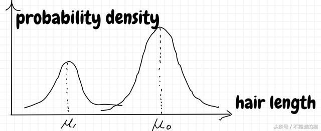
Mixture of Two Gaussians.
Consider a population that is a mixture of two Gaussian distributions. Shown in Fig 2 is this mixture: y = n(x; 3.75, 0.75) + n(x; 6.00, 0.50)
Fig. 2. Sum of Two Gaussians along with 1st and 2nd Derivatives
y = n(x; 3.75, 0.75) + n(x; 6.00, 0.50)
Fig. 3. Heming Lake Pike
Mixture
混合正态分布与基本正态分布或逆高斯分布不同,它的基本思想是:对每一个像素,定义K个状态, 每个状态用一个高斯函数表示,这些状态一部分表示背景的像素值,其余部分则表示前景的像素值。
正态分布的特征
(1)正态分布的曲线特征
正态曲线呈钟型,两头低,中间高,左右对称,曲线与横轴间的面积总等于1。 1、集中性:正态曲线的高峰位于正中央,即均数所在的位置。
2、对称性:正态曲线以均数为中心,左右对称,曲线两端永远不与横轴相交。 3、均匀变动性:正态曲线由均数所在处开始,分别向左右两侧逐渐均匀下降。 4、正态分布有两个参数,即均数μ和标准差σ,可记作N(μ,σ):均数μ决定正态曲线的中心位置;标准差σ决定正态曲线的陡峭或扁平程度。σ越小,曲线越陡峭;σ越大,曲线越扁平。
5、u变换:为了便于描述和应用,常将正态变量作数据转换。
(2)正态曲线下面积分布
1(实际工作中,正态曲线下横轴上一定区间的面积反映该区间的例数占总例数 的百分比,或变量值落在该区间的概率(概率分布)。不同 范围内正态曲线下的面积可用公式计算。
2.几个重要的面积比例 轴与正态曲线之间的面积恒等于1。正态曲线下,横轴区间(μ-σ,μ+σ)内的面积为68.268949%,横轴区间(μ-1.96σ,μ+1.96σ)内的面积为95.449974%,横轴区间(μ-2.58σ,μ+2.58σ)内的面积为99.730020%。 (3)正态分布函数特征
若已知的密度函数(频率曲线)为正态函数(曲线)则称已知曲线服从正态分布,记号 , 。其中μ、σ2 是两个不确定常数,是正态分布的参数,不同的μ、不同的σ2对应不同的正态分布。
(1)μ是正态分布的位置参数,描述正态分布的集中趋势位置。正态分布以X=μ为对称轴,左右完全对称。正态分布的均数、中位数、众数相同,均等于μ。
(2)σ描述正态分布资料数据分布的离散程度,σ越大,数据分布越分散,σ越小,数据分布越集中。 也称为是正态分布的形状参数,σ越大,曲线越扁平,反之,σ越小,曲线越瘦高。
周晓彤
范文五:高斯分布
高斯分布,也称正态分布,又称常态分布。对于随机变量X ,其概率密度函数如图所示。称其分布为高斯分布或正态分布,记为N (μ,σ2),其中为分布的参数,分别为高斯分布的期望和方差。当有确定值时,p(x)也就确定了,特别当μ=0,σ2=1时,X 的分布为标准正态分布。μ正态分布最早由棣莫佛于1730年在求二项分布的渐近公式时得到;后拉普拉斯于1812年研究极限定理时也被引入;高斯(Gauss )则于1809年在研究误差理论时也导出了它。高斯分布的函数图象是一条位于x 轴上方呈钟形的曲线,称为高斯分布曲线,简称高斯曲线。
AWGN (加性高斯白噪声)
加性高斯白噪声(AWGN )从统计上而言是随机无线噪声,其特点是其通信信道上的信号分布在很宽的频带范围内。 高斯白噪声的概念." 白" 指功率谱恒定;
高斯指幅度取各种值
时的概率p (x)是高斯函数.

